DC Motor Speed Control
This example demonstrates multi-domain modeling of a DC motor with PID speed control. The system combines electrical and mechanical dynamics with anti-windup control to handle voltage saturation.
You can also find this example as a single file in the GitHub repository.
The DC motor control system features:
- Electrical subsystem: Armature circuit with resistance, inductance, and back-EMF - Mechanical subsystem: Rotor dynamics with inertia and viscous friction - Anti-windup PID: Prevents integrator windup during voltage saturation - Load disturbances: Tests disturbance rejection capability
DC Motor Physics
A DC motor is a multi-domain electromechanical system where electrical energy is converted to mechanical rotation. The system consists of two coupled subsystems:
Electrical Subsystem (Armature Circuit)
The armature circuit dynamics are governed by Kirchhoff's voltage law:
MATHDISPLAY0ENDMATH
where:
- MATHINLINE3ENDMATH is the applied voltage (control input)
- MATHINLINE4ENDMATH is the armature resistance
- MATHINLINE5ENDMATH is the armature inductance
- MATHINLINE6ENDMATH is the armature current
- MATHINLINE7ENDMATH is the back-EMF (electromotive force)
The back-EMF is proportional to the rotor angular velocity:
MATHDISPLAY1ENDMATH
where MATHINLINE8ENDMATH is the back-EMF constant and MATHINLINE9ENDMATH is the angular velocity. Rearranging for the current derivative:
MATHDISPLAY2ENDMATH
Mechanical Subsystem (Rotor Dynamics)
The rotor dynamics are described by Newton's second law for rotation:
MATHDISPLAY0ENDMATH
where:
- MATHINLINE4ENDMATH is the rotor moment of inertia
- MATHINLINE5ENDMATH is the electromagnetic torque
- MATHINLINE6ENDMATH is the viscous friction torque
- MATHINLINE7ENDMATH is the external load torque
The electromagnetic torque is proportional to the armature current:
MATHDISPLAY1ENDMATH
where MATHINLINE8ENDMATH is the torque constant. The friction torque is proportional to angular velocity:
MATHDISPLAY2ENDMATH
where MATHINLINE9ENDMATH is the viscous friction coefficient. The complete mechanical equation becomes:
MATHDISPLAY3ENDMATH
Electromechanical Coupling
The two subsystems are bidirectionally coupled:
- Electrical → Mechanical: Current MATHINLINE0ENDMATH produces torque MATHINLINE1ENDMATH
- Mechanical → Electrical: Angular velocity MATHINLINE2ENDMATH produces back-EMF MATHINLINE3ENDMATH
This coupling creates natural feedback: as the motor speeds up, the back-EMF increases, which opposes the applied voltage and reduces current. At steady-state with no load, the motor reaches an equilibrium where the back-EMF nearly balances the applied voltage.
PID Speed Control
To control the motor speed, we use a PID (Proportional-Integral-Derivative) controller. The control law is:
MATHDISPLAY0ENDMATH
where MATHINLINE2ENDMATH is the speed error.
Anti-Windup Mechanism
Since the applied voltage is physically limited (MATHINLINE3ENDMATH), the integrator can "wind up" during saturation, causing overshoot. The anti-windup mechanism modifies the integral term:
MATHDISPLAY1ENDMATH
where MATHINLINE4ENDMATH is the anti-windup gain. When saturation occurs, the feedback term prevents further integration.
Import and Setup
First let's import the required classes and blocks:
Motor Parameters
We define realistic parameters for a small DC motor:
Source Signals
Define the speed setpoint with step changes and load torque disturbances using subsequent step signals with the StepSource .
System Definition
Now we construct the multi-domain system with separate electrical and mechanical subsystems:
The connections implement the coupled electrical-mechanical dynamics with feedback control:
Simulation Setup and Execution
We initialize the simulation with the RKCK54 solver (Runge-Kutta Cash-Karp 5th order with adaptive step size):
19:04:12 - INFO - LOGGING (log: True)
19:04:12 - INFO - BLOCKS (total: 17, dynamic: 3, static: 14, eventful: 2)
19:04:12 - INFO - GRAPH (nodes: 17, edges: 22, alg. depth: 6, loop depth: 0, runtime: 0.191ms)
19:04:12 - INFO - STARTING -> TRANSIENT (Duration: 30.00s)
19:04:12 - INFO - --------------------   1% | 0.1s<6.8s | 871.3 it/s
19:04:13 - INFO - ###-----------------  15% | 1.1s<4.8s | 844.7 it/s
19:04:14 - INFO - ####----------------  20% | 1.5s<6.8s | 823.4 it/s
19:04:15 - INFO - ######--------------  32% | 2.5s<3.7s | 894.7 it/s
19:04:15 - INFO - ########------------  40% | 3.0s<3.9s | 1004.5 it/s
19:04:16 - INFO - ##########----------  54% | 4.0s<2.5s | 865.7 it/s
19:04:16 - INFO - ############--------  60% | 4.3s<2.5s | 768.2 it/s
19:04:17 - INFO - ##############------  74% | 5.3s<1.8s | 829.0 it/s
19:04:18 - INFO - ################----  80% | 5.7s<1.3s | 807.4 it/s
19:04:19 - INFO - ###################-  96% | 6.7s<0.2s | 890.4 it/s
19:04:19 - INFO - #################### 100% | 7.0s<--:-- | 835.2 it/s
19:04:19 - INFO - FINISHED -> TRANSIENT (total steps: 5837, successful: 4938, runtime: 7041.33 ms)
Results
Let's plot the speed tracking and electrical signals:
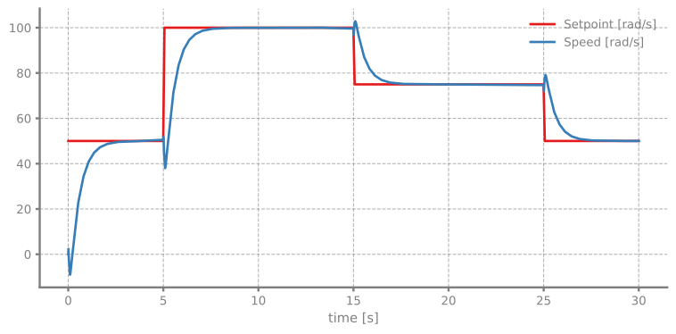
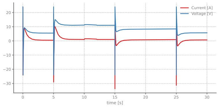
This example demonstrates PathSim's capability to model multi-domain systems with bidirectional coupling:
- Multi-domain physics: Electrical and mechanical subsystems with natural coupling through back-EMF and electromagnetic torque - Advanced control: :class: controller handles actuator saturation gracefully - Disturbance rejection: Controller compensates for external load torques - Realistic dynamics: Captures transient and steady-state behavior of real DC motors
The model accurately represents the energy conversion and control challenges in electromechanical systems, making it useful for motor controller design and analysis.