This example is interactive. Click the play button on any cell to execute it, or run all cells in sequence.

SAR ADC

Simulation of a Successive Approximation Register ADC with custom block creation.

You can also find this example as a single file in the GitHub repository.

Successive Approximation Register (SAR) ADC Principle

A SAR ADC converts analog signals to digital using a binary search algorithm:

Sample the input voltage
Test the MSB (Most Significant Bit) by comparing to DAC output
Keep the bit if comparison succeeds, discard if it fails
Repeat for each bit from MSB to LSB
Output the complete digital word

This requires N comparisons for N bits, making it efficient for medium-speed, medium-resolution applications (10-18 bits, up to several MHz).

Custom SAR Logic Block

We'll implement the SAR control logic as a custom block using PathSim's event system.

This example shows how to create custom blocks by extending the Block class and using Schedule events for discrete-time logic.

Python

Creating a Custom SAR Logic Block

This is one of PathSim's powerful features - you can create custom blocks with complex behavior. The SAR block:

Uses scheduled events to step through bits
Implements the binary search algorithm
Outputs N parallel digital signals (one per bit)

Python

System Parameters

We'll use:

8-bit resolution
50 Hz sampling frequency
Modulated sine wave as input signal

Python

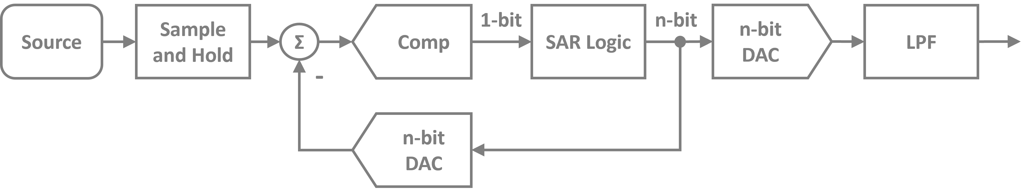
Block Diagram Setup

The system consists of:

src: Modulated sine wave source
sah: Sample & Hold to freeze input during conversion
sub: Subtractor (input - DAC)
cpt: Comparator
sar: Custom SAR logic
dac1: Fast DAC for comparison (updates every bit)
dac2: Output DAC (updates every sample)
lpf: Lowpass filter for reconstruction

Python

Connections

The connections form the SAR ADC loop. Notice how the 8 digital bits from SAR connect to both DACs in parallel.

Python

Simulation

We run the simulation with an adaptive solver that can handle the discrete-time events efficiently.

Python

12:44:01 - INFO - LOGGING (log: True)
12:44:01 - INFO - BLOCKS (total: 9, dynamic: 1, static: 8, eventful: 5)
12:44:01 - INFO - GRAPH (nodes: 9, edges: 27, alg. depth: 3, loop depth: 0, runtime: 0.141ms)
12:44:01 - INFO - STARTING -> TRANSIENT (Duration: 1.00s)
12:44:01 - INFO - --------------------   1% | 0.0s<0.7s | 1713.6 it/s
12:44:01 - INFO - ####----------------  20% | 0.2s<1.2s | 1890.2 it/s
12:44:02 - INFO - ########------------  40% | 0.4s<0.4s | 1948.4 it/s
12:44:02 - INFO - ############--------  60% | 0.7s<0.5s | 1618.6 it/s
12:44:02 - INFO - ################----  80% | 0.9s<0.1s | 2590.3 it/s
12:44:02 - INFO - #################### 100% | 1.0s<--:-- | 2850.0 it/s
12:44:02 - INFO - FINISHED -> TRANSIENT (total steps: 2124, successful: 2034, runtime: 1046.22 ms)

Results

The plots show:

src: Original analog input
sah: Sampled and held signal
dac1: Fast DAC during conversion (shows binary search)
dac2: Output DAC (quantized signal)
lpf: Reconstructed signal after filtering

Notice how dac1 shows the successive approximation steps within each sample period!

Python