This example is interactive. Click the play button on any cell to execute it, or run all cells in sequence.

Pendulum

Simulation of a nonlinear mathematical pendulum.

You can also find this example as a single file in the GitHub repository.

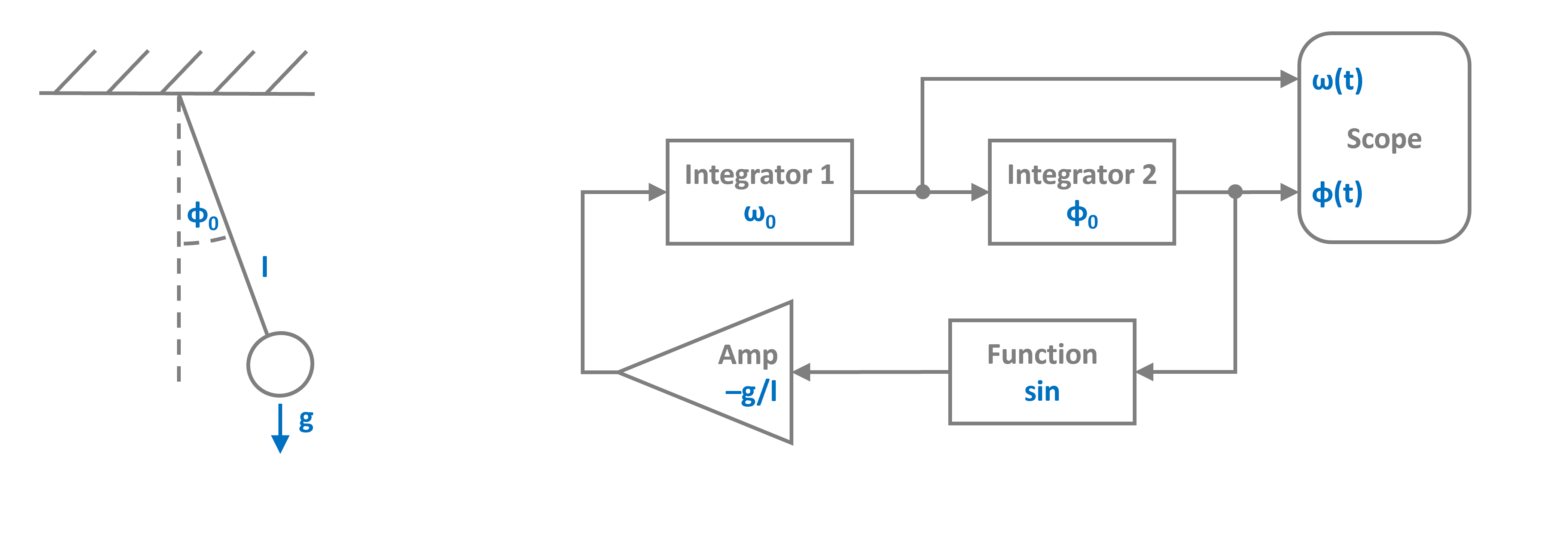
Above we have both the mechanical mode, which is a weight dangling from a string with length l and diverted by some initial angle, as well as the block diagram representation of the equation of motion to the right.

The equation of motion of the system is a nonlinear second order ODE:

MATHDISPLAY0ENDMATH

Lets transition to Python by importing the components we need to model the system from PathSim

Python

and define the system parameters. Here we choose an initial angle that is close to the pendulum beeing at the top:

Python

We can directly translate the block diagram above to PathSim blocks and connections:

Python

The simulation is initialized with the blocks and connections. In this case we dont use the default solver but an adaptive integrator RKCK54 to ensure accuracy. Its an adaptive runge-kutta method from Cash and Karp, similar to Matlabs ode45, which is from Dormand and Prince and RKDP54 in PathSim. The tolerances we set here, are also for the integrator. The adaptive method controls the timestep such that the local truncation error (lte) stays below the set tolerances.

Python

12:43:55 - INFO - LOGGING (log: True)
12:43:55 - INFO - BLOCKS (total: 5, dynamic: 2, static: 3, eventful: 0)
12:43:55 - INFO - GRAPH (nodes: 5, edges: 6, alg. depth: 3, loop depth: 0, runtime: 0.070ms)

Finally we can run the simulation for some number of seconds and see what happens.

Python

12:43:55 - INFO - STARTING -> TRANSIENT (Duration: 15.00s)
12:43:55 - INFO - --------------------   1% | 0.0s<0.2s | 1201.4 it/s
12:43:55 - INFO - ####----------------  20% | 0.0s<0.1s | 2062.4 it/s
12:43:55 - INFO - ########------------  40% | 0.0s<0.0s | 2197.3 it/s
12:43:55 - INFO - ############--------  60% | 0.1s<0.0s | 2748.1 it/s
12:43:55 - INFO - ################----  80% | 0.1s<0.0s | 2210.8 it/s
12:43:55 - INFO - #################### 100% | 0.1s<--:-- | 2483.1 it/s
12:43:55 - INFO - FINISHED -> TRANSIENT (total steps: 207, successful: 174, runtime: 98.50 ms)

Since we are using an adaptive integrator, it might be interesting to also look at the timesteps the simulation takes. To do this, we just get the times from the scope and compute the differences:

Python

We can clearly see that the integrator takes smaller steps when the pendulum gets closer to regions where the solution trajectory is more dynamic to keep the local truncation error below the tolerances.