This example is interactive. Click the play button on any cell to execute it, or run all cells in sequence.

Noisy Amplifier

Simulation of a nonlinear, noisy, and band-limited amplifier model.

The most simplistic model for an amplifier is just the product of a signal with some factor (gain). But we all know, real amplifiers are noisy and nonlinear. Internal physical processes or fluctiations in the power supply produce noise and if the amplitudes get too big, we run into saturations.

PathSim implements a number (WhiteNoiseSource and PinkNoiseSource) of broadband noise generators that produce accurate frequency domain noise spectra but for transient analysis.

In this example we are bringing that together to implement a simple model of a nonlinear, noisy and band limited amplifier shown in the figure below:

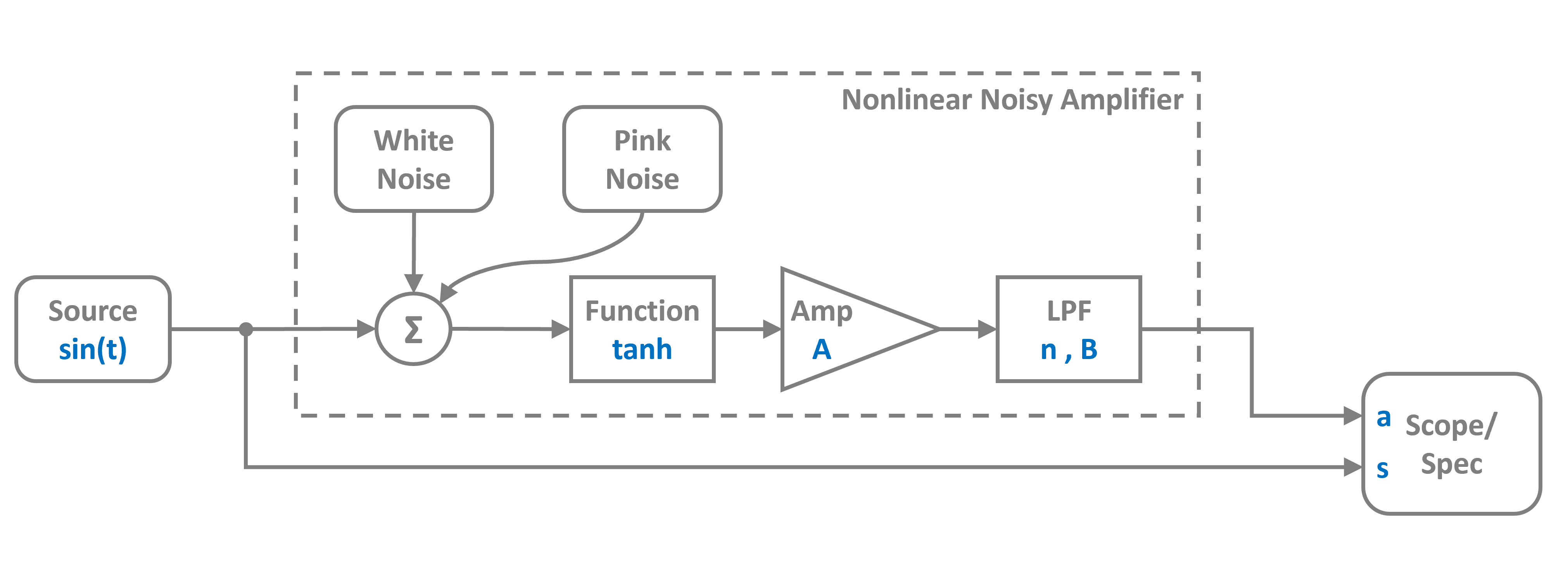
block diagram of nonlinear noisy amplifier

Python

Noisy Amplifier Model as Subsystem

The nonlinear amplifier model is defined as a Subsystem, implementing the gain as an elementary Amplifier block, the saturation (nonlinearity) as a Function block, wrapping a hyperbolic tangent and a ButterworthLowpassFilter for the frequency dependency. On top of that, two noise sources (WhiteNoiseSource and PinkNoiseSource) are added to the input of the model.

Python

Main System (Top Level)

The amplifier model is ready, we connect an sinusoidal source to its input and a spectrum analyzer (Spectrum) and Scope to its output.

Python

12:43:51 - INFO - LOGGING (log: True)
12:43:51 - INFO - BLOCKS (total: 4, dynamic: 2, static: 2, eventful: 0)
12:43:51 - INFO - GRAPH (nodes: 4, edges: 5, alg. depth: 1, loop depth: 0, runtime: 0.035ms)

Simulation

Lets run the simulation for some duration. Here 100us, 20 periods of the sinusoidal source.

Python

12:43:51 - INFO - STARTING -> TRANSIENT (Duration: 0.00s)
12:43:51 - INFO - --------------------   1% | 0.0s<1.4s | 2305.7 it/s
12:43:52 - INFO - ####----------------  20% | 0.3s<1.1s | 2374.5 it/s
12:43:52 - INFO - ########------------  40% | 0.6s<0.8s | 2419.7 it/s
12:43:52 - INFO - ############--------  60% | 0.8s<0.5s | 2459.3 it/s
12:43:52 - INFO - ################----  80% | 1.1s<0.3s | 2393.8 it/s
12:43:53 - INFO - #################### 100% | 1.4s<--:-- | 2456.6 it/s
12:43:53 - INFO - FINISHED -> TRANSIENT (total steps: 3334, successful: 3334, runtime: 1396.95 ms)

Results

We can read the time series results and see that we get the expected amplified sinusoid. The noise parameters we chose are pretty big, so we can see the fluctuations.

Python

In the frequency domain we can see the second peak in te spectrum of the output signal. This indicates the nonlinearity.

Python