This example is interactive. Click the play button on any cell to execute it, or run all cells in sequence.

Kalman Filter

This example demonstrates the Kalman filter in PathSim for optimal state estimation of a linear dynamical system from noisy measurements. The filter recursively estimates the state of a moving object by combining predictions from a system model with noisy sensor measurements.

You can also find this example as a single file in the GitHub repository.

block diagram with kalman filter for state estimation

Import and Setup

First let's import the required classes and blocks:

Python

System Parameters

We simulate a simple object moving with constant velocity. The true system has a velocity of 2 m/s, but we can only measure its position with noisy sensors. The Kalman filter will estimate both position and velocity from the noisy position measurements.

Python

Kalman Filter Configuration

The Kalman filter requires several matrices:

F: State transition matrix (how the state evolves)
H: Measurement matrix (what we can observe)
Q: Process noise covariance (model uncertainty)
R: Measurement noise covariance (sensor uncertainty)
x0: Initial state estimate
P0: Initial error covariance

Python

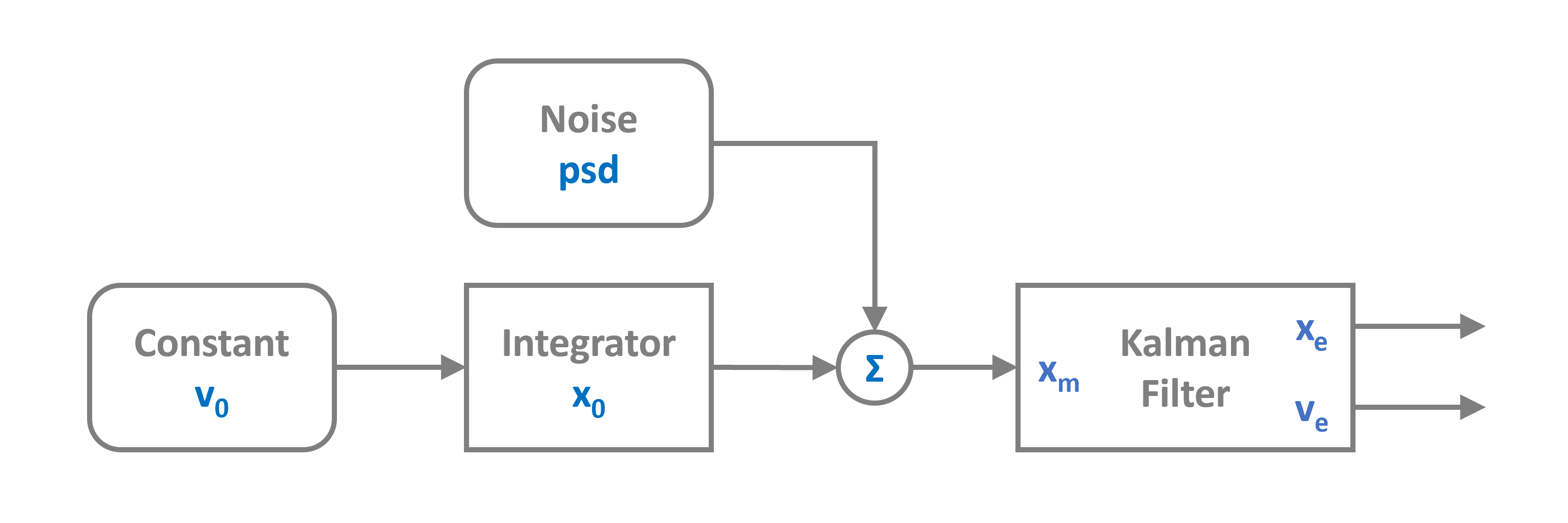
System Definition

Now we construct the complete system including:

The true system (constant velocity integrator)
Noisy measurement sensor
Kalman filter for state estimation

Python

The WhiteNoise block adds Gaussian noise to the true position measurement. The KalmanFilter processes these noisy measurements to estimate both position and velocity.

Python

Simulation Setup and Execution

Python

12:43:44 - INFO - LOGGING (log: True)
12:43:44 - INFO - BLOCKS (total: 8, dynamic: 1, static: 7, eventful: 0)
12:43:44 - INFO - GRAPH (nodes: 8, edges: 9, alg. depth: 2, loop depth: 0, runtime: 0.080ms)
12:43:44 - INFO - STARTING -> TRANSIENT (Duration: 20.00s)
12:43:44 - INFO - --------------------   1% | 0.0s<0.4s | 4764.4 it/s
12:43:44 - INFO - ####----------------  20% | 0.1s<0.4s | 4342.3 it/s
12:43:44 - INFO - ########------------  40% | 0.2s<0.3s | 4487.6 it/s
12:43:44 - INFO - ############--------  60% | 0.3s<0.2s | 4580.2 it/s
12:43:44 - INFO - ################----  80% | 0.4s<0.1s | 3952.6 it/s
12:43:45 - INFO - #################### 100% | 0.5s<--:-- | 6627.6 it/s
12:43:45 - INFO - FINISHED -> TRANSIENT (total steps: 2000, successful: 2000, runtime: 455.49 ms)

Results: State Tracking

Let's visualize how well the Kalman filter tracks the true position and velocity:

Python

Estimation Error Analysis

Now let's quantify the estimation accuracy by computing and plotting the absolute errors:

Python