This example is interactive. Click the play button on any cell to execute it, or run all cells in sequence.

Elastic Pendulum

Simulation of an elastic pendulum combining spring and pendulum dynamics.

You can also find this example as a standalone Python file in the GitHub repository.

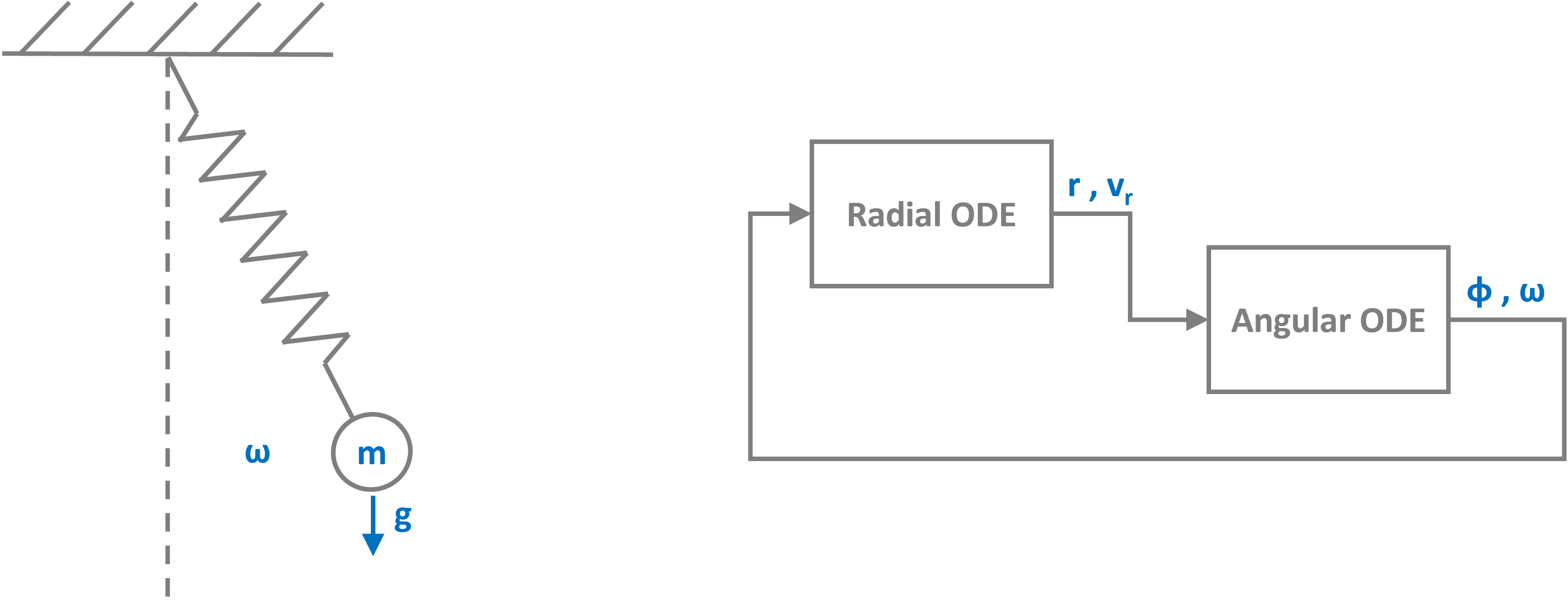
We implement this system im pathsim through two separate ODE blocks, one for the radial and one for the angular dynamics. The connections between the blocks represent the coupling through the forces.

Python

Next, the two ODE blocks are defined through their right hand side function. For the radial component this is the following set of odes with the centrifugal force coupling and the acceleration through gravity:

MATHDISPLAY0ENDMATH

MATHDISPLAY1ENDMATH

Python

For the angular component we have the following odes:

MATHDISPLAY0ENDMATH

MATHDISPLAY1ENDMATH

Python

For straight forward plotting and evaluation it makes sense to convert from polar to cartesian coordinates. For this, we use a Function block. It can be defined through a decorator which makes it super compact:

Python

Next, define the connections (Connection) between the two blocks...

Python

... initialize the Simulation with the blocks and connections. The dynamics of this system can be very chaotic, so it makes sense to use an adaptive timestep ode solver such as RKBS32:

Python

12:43:41 - INFO - LOGGING (log: True)
12:43:41 - INFO - BLOCKS (total: 5, dynamic: 2, static: 3, eventful: 1)
12:43:41 - INFO - GRAPH (nodes: 5, edges: 9, alg. depth: 2, loop depth: 0, runtime: 0.066ms)

Python

12:43:41 - INFO - STARTING -> TRANSIENT (Duration: 10.00s)
12:43:41 - INFO - --------------------   1% | 0.0s<0.8s | 2465.8 it/s
12:43:41 - INFO - ####----------------  20% | 0.2s<0.6s | 2514.3 it/s
12:43:41 - INFO - ########------------  40% | 0.3s<0.2s | 5139.6 it/s
12:43:41 - INFO - ############--------  60% | 0.5s<0.3s | 2555.1 it/s
12:43:42 - INFO - ################----  80% | 0.7s<0.1s | 3198.6 it/s
12:43:42 - INFO - #################### 100% | 0.9s<--:-- | 2613.5 it/s
12:43:42 - INFO - FINISHED -> TRANSIENT (total steps: 2130, successful: 2083, runtime: 902.88 ms)

One of pathsims convenient features is that each block is physicalized. This means the Scope block records the signals internally and the data can be read and plotted through its local methods directly:

Python

We can clearly see the mass jumping back and forth, driventhrough the contracting spring at each swing:

Python