This example is interactive. Click the play button on any cell to execute it, or run all cells in sequence.

Coupled Oscillators

Simulation of two coupled damped harmonic oscillators using ODE blocks.

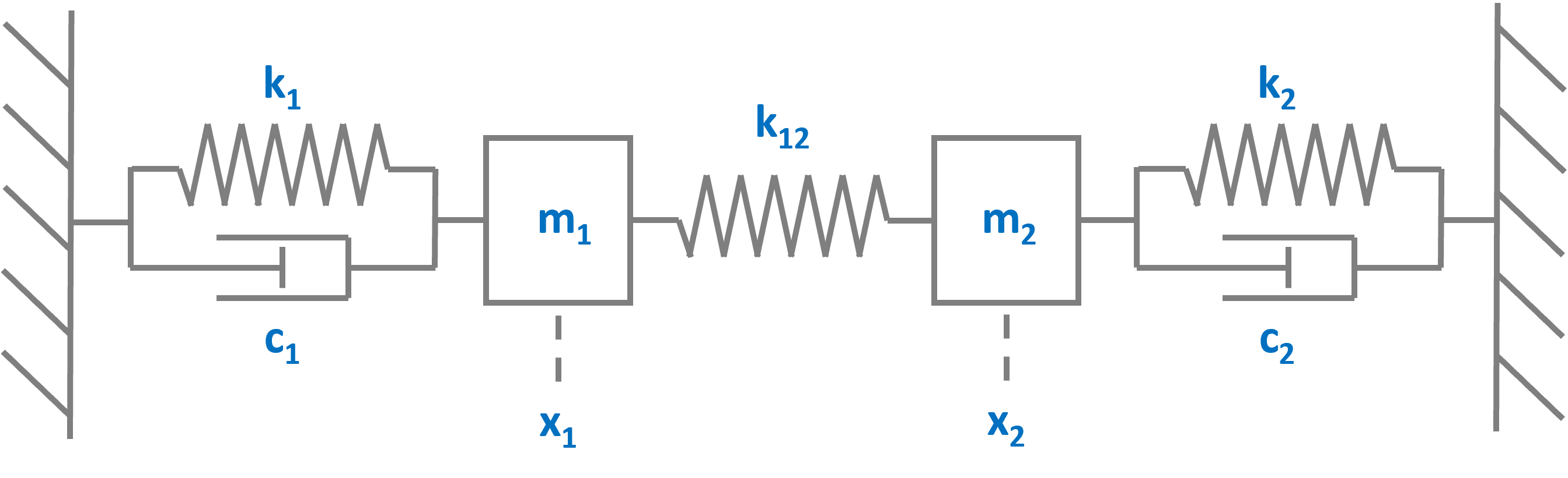
The equations of motion for the coupled system are:

m_1 \ddot{x}_1 = -k_1 x_1 - c_1 \dot{x}_1 - F_e m_2 \ddot{x}_2 = -k_2 x_2 - c_2 \dot{x}_2 + F_e

With the force-coupling given as:

F_e = k_{12}(x_1 - x_2)

where :math:`m_1, m_2` are the masses, :math:`k_1, k_2` are the spring constants, :math:`c_1, c_2` are the damping coefficients, and :math:`k_{12}` is the coupling spring constant between the two oscillators, leading to external forces :math:`F_e`.

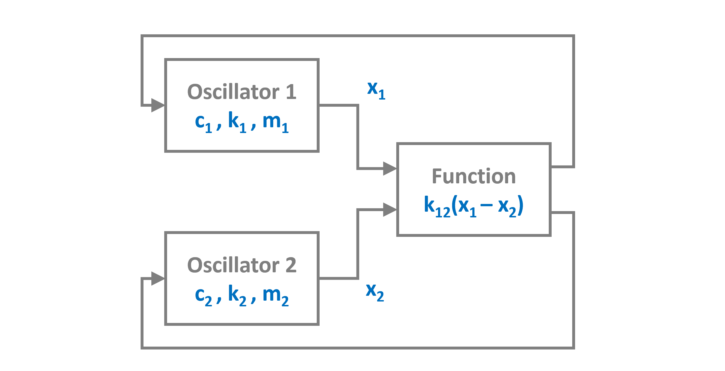
As a block diagram it would look like this:

block diagram of two coupled ODE blocks with Scope

Now let's implement this system in PathSim:

First let's import the Simulation and Connection classes and the required blocks from the block library:

Python

System Parameters

Next, let's define the system parameters:

Python

Block Construction

Now we define the differential equations for each oscillator and create the ODE blocks:

Each ODE block takes a function that defines the right-hand side of the differential equation, an initial condition, and optionally a Jacobian for improved convergence with implicit solvers.

Python

Connections

Now we connect the blocks. The key aspect of this system is the coupling between the two oscillators:

The Connection class defines the signal flow between blocks. Each oscillator sends its state to the other oscillator as input, creating the coupling. We also connect both oscillators to the Scope for visualization.

Python

Simulation Setup

Finally, we create the simulation:

We instantiate the Simulation with the blocks and connections. For this non-stiff system, the default SSPRK22 solver (a 2nd order explicit Runge-Kutta method) works well.

Python

12:43:30 - INFO - LOGGING (log: True)
12:43:30 - INFO - BLOCKS (total: 5, dynamic: 2, static: 3, eventful: 0)
12:43:30 - INFO - GRAPH (nodes: 5, edges: 7, alg. depth: 2, loop depth: 0, runtime: 0.060ms)

Running the Simulation

Now let's run the simulation and visualize the results:

Python

12:43:30 - INFO - STARTING -> TRANSIENT (Duration: 75.00s)
12:43:30 - INFO - RESET (time: 0.0)
12:43:30 - INFO - --------------------   1% | 0.0s<0.8s | 8819.5 it/s
12:43:30 - INFO - ####----------------  20% | 0.2s<0.7s | 8787.9 it/s
12:43:30 - INFO - ########------------  40% | 0.4s<0.6s | 7979.7 it/s
12:43:30 - INFO - ############--------  60% | 0.5s<0.3s | 9163.8 it/s
12:43:31 - INFO - ################----  80% | 0.7s<0.2s | 7374.0 it/s
12:43:31 - INFO - #################### 100% | 0.9s<--:-- | 7795.5 it/s
12:43:31 - INFO - FINISHED -> TRANSIENT (total steps: 7500, successful: 7500, runtime: 924.20 ms)

Analysis

The plot shows the position of both oscillators over time. Notice how:

Energy Transfer: The initially displaced oscillator 1 transfers energy to oscillator 2 through the coupling spring.
Damped Motion: Both oscillators gradually lose energy due to damping, eventually settling to rest.
Coupled Dynamics: The motion of each oscillator is influenced by the other, creating a complex interplay.

This example demonstrates how PathSim can elegantly handle coupled differential equations using multiple ODE blocks that exchange information through connections, making it easy to model systems with interacting components.