This example is interactive. Click the play button on any cell to execute it, or run all cells in sequence.

Bouncing Pendulum

This example demonstrates a hybrid system combining continuous pendulum dynamics with discrete bounce events. The pendulum swings until it hits the ground (zero angle), at which point it bounces back with reduced energy.

You can also find this example as a single file in the GitHub repository.

This example showcases:

- Nonlinear pendulum dynamics with ZeroCrossing event detection - State transformations at discrete events (angular velocity reversal) - Automatic differentiation through hybrid systems with the Value class - Sensitivity analysis of the bounce elasticity parameter

First let's import the Simulation and Connection classes along with the required blocks and event manager:

Python

System Dynamics

The mathematical pendulum is governed by the nonlinear differential equation:

MATHDISPLAY0ENDMATH

where:

MATHINLINE1ENDMATH is the angle from vertical
MATHINLINE2ENDMATH is gravitational acceleration
MATHINLINE3ENDMATH is the pendulum length

The bounce event occurs when MATHINLINE4ENDMATH (pendulum hits the ground), at which point the angular velocity reverses with a loss factor.

Python

Note that we wrap the bounceback coefficient b in a Value instance to enable automatic differentiation. This allows us to compute sensitivities of the system response with respect to this parameter.

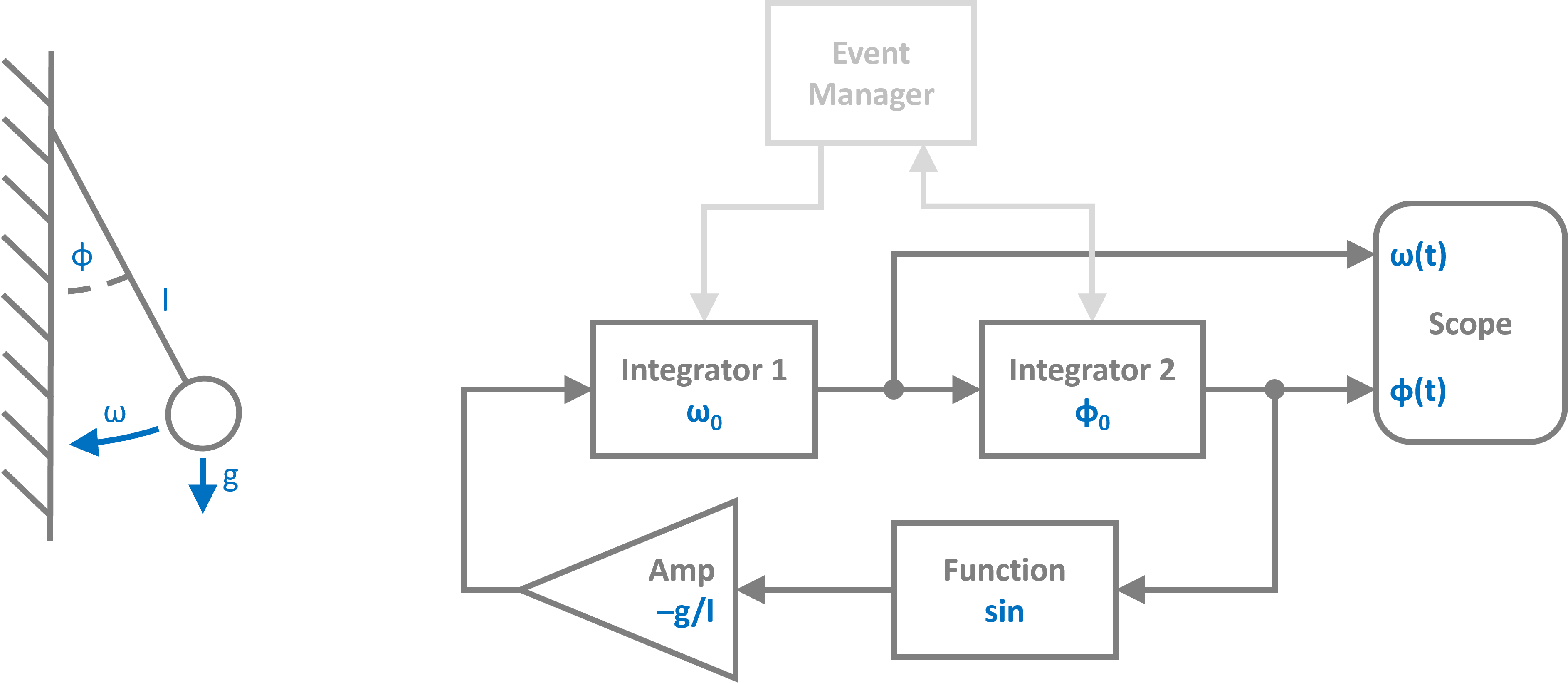
schematic of a bouncing pendulum against a wall

Block Diagram Construction

We construct the system from basic blocks:

Python

Event Detection and Action

We define a ZeroCrossing event to detect when the pendulum hits the ground ($\phi = 0$). The event function monitors the angle, and the action function reverses the angular velocity with an energy loss factor.

Python

The engine.set() method allows direct manipulation of block states during event actions. This is crucial for implementing the discontinuous velocity change at the bounce.

We initialize the simulation with the RKCK54 solver for accurate integration of the nonlinear dynamics:

Python

12:43:20 - INFO - LOGGING (log: True)
12:43:21 - INFO - BLOCKS (total: 5, dynamic: 2, static: 3, eventful: 0)
12:43:21 - INFO - GRAPH (nodes: 5, edges: 6, alg. depth: 3, loop depth: 0, runtime: 0.070ms)

Now let's run the simulation:

Python

12:43:21 - INFO - STARTING -> TRANSIENT (Duration: 15.00s)
12:43:21 - INFO - --------------------   1% | 0.0s<0.2s | 1176.4 it/s
12:43:21 - INFO - ####----------------  20% | 0.0s<0.1s | 2118.0 it/s
12:43:21 - INFO - ########------------  40% | 0.1s<0.1s | 2220.5 it/s
12:43:21 - INFO - ############--------  60% | 0.1s<0.0s | 2285.1 it/s
12:43:21 - INFO - ################----  80% | 0.1s<0.0s | 2227.5 it/s
12:43:21 - INFO - #################### 100% | 0.2s<--:-- | 2178.3 it/s
12:43:21 - INFO - FINISHED -> TRANSIENT (total steps: 327, successful: 254, runtime: 164.45 ms)

Results

Let's plot the angular velocity and angle over time, marking the bounce events:

Python

The plot shows:

The angle oscillates between 0 and some maximum value that decreases over time
The angular velocity reverses sign at each bounce (vertical dashed lines)
Energy is progressively lost with each bounce, leading to smaller oscillations